Consider any species that typically gives birth to one offspring per mating, and that within that species is any simply-inherited trait with a dominant ‘A’ allele and a recessive ‘a’ allele.

Now consider four individuals of that species, all with known genotypes: a heterozygous dominant male (’Aa’), a homozygous dominant female (’AA’), a heterozygous dominant female (’Aa’), and a homozygous recessive female (’aa’). Assume a genetic test doesn’t exist. The mating outcomes of the male over each of these females can be summarised as:

We know with certainty which of the progeny are recessive (’aa’) just by looking at them. We also know with certainty that the genotypes of the homozygous recessive female’s offspring that aren’t themselves recessive must be heterozygous dominant (’Aa’). But how do we know which of the others are homozygous (’AA’) or heterozygous (’Aa’) dominant?

All we can know for sure is that the probability of an ‘AA’ genotype resulting when our male is crossed with a known ‘AA’ female is 1 in 2, or 0.5. Likewise the probability of an ‘Aa’ genotype from the same mating is 0.5. The probability of an ‘AA’ genotype with a known ‘Aa’ mating is 1 in 4, or 0.25, and of an ‘Aa’ genotype is 2 in 4, or 0.5.

We can calculate these probabilities as we already know the genotypes of the parents. But if we don’t know the genotypes of the parents, we must then rely on what we know about population genetics, and work with the probabilities of certain genotypes being in the population as a whole.

Back in The Effect of Mating Systems on Gene and Genotypic Frequencies: Outbreeding, we saw how Punnet squares can be used to calculate genotypic frequencies in the offspring, given the gene frequencies in the starting population.

We can use Punnet squares similarly to calculate the probabilities of which genotypes are likely to be in the offspring, given the known probabilities of those genotypes being in the starting population.

Instead of p and q representing gene frequencies, let them now represent the probabilities that an animal will contribute a dominant allele or a recessive allele.

Here, p is the probability that ‘A’ is passed to the progeny, and q is the probability that ‘a’ is passed to the progeny.

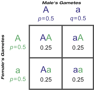
If we know a male is ‘Aa’ then both p and q are 0.5. There is a 50% chance that any of his gametes picked at random will have an ‘A’ or ‘a’ allele.

If we don’t know for sure whether any particular female is ‘AA’ or ‘Aa’ we must work with the probabilities of these alleles being in the population of females as a whole.

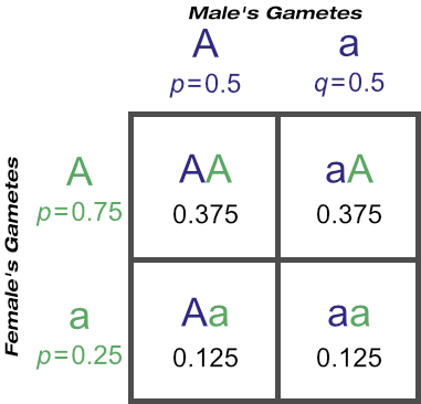
Revisiting the first Punnet square above, of an ‘Aa’ male and ‘AA’ female mating, you can see that half the progeny are expected to be ‘AA’ and half expected to be ‘Aa’. Extrapolating this outcome to a larger population of females, half will similarly be expected to be ‘AA’ and the other half ‘Aa’.

From this, there are expected to be three ‘A’ alleles to every ‘a’ in that wider population, or three in four. Thus the probability of ‘A’ being present in the population is p = 0.75. And from this we know that the probability of ‘a’ being present is q = 0.25.

On crossing our known ‘Aa’ male with any female from a known ‘AA’ dam:

You’ll see the probability of a homozygous recessive genotype (’aa’) from mating a known heterozygous dominant male to females from known ‘AA’ dams is 0.125, or one in eight. This of course means the probability of producing a dominant genotype (whether ‘AA’ or ‘Aa’) is seven in eight (0.375 + 0.375 + 0.125 = 0.875 = ⁷/₈). Three of those are expected to be homozygous dominant (’AA’) and four are expected to be heterozygous dominant (’Aa’).

This same method can be used to work out the probabilities of any genotype from any starting genotypes.

For example, continuing with the middle Punnet square at top, the probabilities of mating outcomes from crossing those progeny from known ‘Aa’ dams with a known ‘Aa’ animal is:

(This is the same result as simply crossing two known ‘Aa’ animals.)

From the third, end Punnet square at top we can see that crossing a known ‘Aa’ male with any ‘aa’ homozygous recessive female would result in half ‘Aa’ and half ‘aa’ progeny on average. Let’s step through this one mathematically, even though the progeny genotypes will be known by sight:

We already know the probability of an ‘Aa’ animal contributing ‘A’ or ‘a’ is p = q = 0.5.
The probability of an ‘aa’ animal contributing an ‘A’ gamete is p = 0, and the probability of contributing an ‘a’ allele is q = 1.

Thus the probability of any ‘AA’ genotypes from an ‘Aa’ × ’aa’ cross is:
the probability of an ‘A’ allele from the ‘Aa’ genotype and the probability of an ‘A’ allele from the ‘aa’ genotype, or
0.5 × 0 = 0

Similarly, the probaility of any ‘aa’ genotypes from an ‘Aa’ × ’aa’ cross is
the probability of an ‘a’ allele from the ‘Aa’ genotype and the probability of an ‘a’ allele from the ‘aa’ genotype, or
0.5 × 1 = 0.5.

And lastly, the probability of any ‘Aa’ genotypes is
the probability of an ‘A’ allele from the ‘Aa’ genotype and the probability of an ‘a’ allele from the ‘aa’ genotype, or
0.5 × 1 = 0.5

It’s all well and good to be able to calculate these probabilities, but there’s one more number we need, and that is the number of births required to be sure a tested animal is not a carrier of a recessive gene. This number will differ depending on the type of mating, and we will go over that in more detail later.

But first a small diversion to discuss the practicalities and limitations of test matings — our topic for next week!