The Better Breeding Blog Breed Better Animals

Last week we saw how crossbreeding — or more accurately, random matings and/or matings between unrelated populations — do not change gene and genotypic frequencies from generation to generation. This phenomenon is known as the Hardy-Weinberg Equlibrium, named after its co-discovers the English mathematician Godfrey Hardy and the German obstetrician-gynecologist Wilhelm Weinberg.

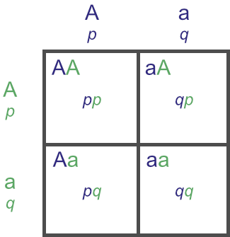
The Hardy-Weinberg Equilbrium states that gene and genotypic frequencies will not change from generation to generation, assuming random matings in the absence of external forces. It further states that, given two alleles at a locus with gene frequencies p and q within a population, that the genotypic frequencies of those alleles will be P = p², H = 2pq, and Q = q².

(This second statement is more clear with the following Punnet square:

Remember that p and q are the gene frequencies of the ‘A’ and ‘a’ alleles respectively. P, H and Q are the genotypic frequencies of the ‘AA’, ‘Aa’ and ‘aa’ genotypes respectively. Thus:
P (or ‘AA’) = p × p = p²,
H (or ‘Aa’) = (p × q) + (q × p) = (pq) + (qp) = (pq) + (pq) = 2 × (pq) = 2pq, and
Q (or ‘aa’) = q × q = q².)

Let’s go back to the first statement, that gene and genotypic frequencies will not change from generation to generation, and revisit the qualifying part: ‘assuming random matings in the absence of external forces’.

What are the external forces that affect a Hardy-Weinberg Equilibrium? The following are all known, and apply to both wild populations and breeding programmes:

Selection. We’ve shown in this post how selecting for particular alleles changes their frequencies within a population. An example in a breeding programme would be the selection for polled cattle, where it’s desirable to increase the frequency of the ‘P’ (polled, or hornless) allele to 1 (100%). A classic example in nature is the evolution of the peppered moth in Manchester, UK, during the Industrial Revolution. Prior to this period, peppered moths were white-bodied with a ‘peppering’ of brown spots and splotches all over. This colouring was an effective camouflage against tree trunks in a clean environment. Sometime after 1811 however, a new, predominant form arose that was solid brown. This colouring was a more effective camouflage against the soot-covered trunks in polluted areas.

Gene mutations. This is a very rare event, but changes during DNA replication can alter genes and create new alleles. The mere presence of a new allele in a population is enough to shift gene and genotypic frequencies accordingly. One example of this is the explosion of budgerigar colour mutations from the late 1800s on — where once all pet budgies had the same green and yellow and blue markings, there is now a plethora of colours. The popularity of this little Australian parrot led to a population increase worldwide, which increased the chances of rare mutations affecting colours and markings appearing. Breeders would then deliberately select for these, ultimately increasing the gene and genotypic frequencies throughout the worldwide population of budgerigars. Likewise, the many colour varieties of the North American corn snake similarly arose from selective breeding that deliberately shifted frequencies away from those in the wild population.

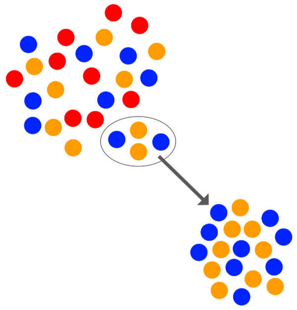
Migration in and out of a population. The movement of animals in and out of a population can change frequencies significantly, especially if large numbers of very different animals are introduced. An example was briefly mentioned here, where in the 1990s, the introduction to Australia of alpacas with greater density and coverage changed the appearance of the national herd in just a few years.

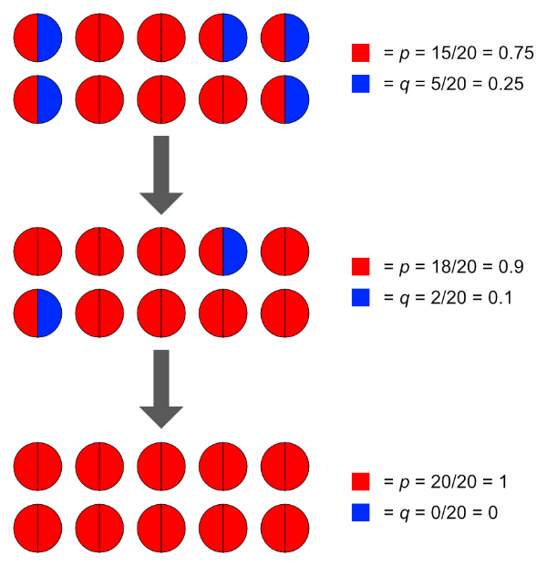
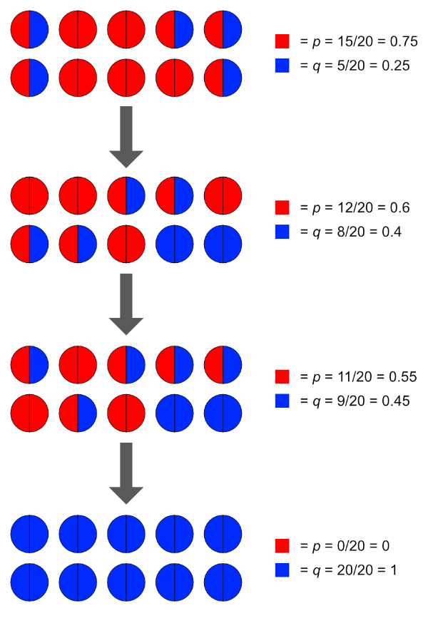
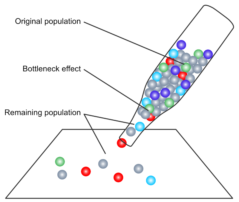
Small population size. Small populations quickly become inbred, and inbred populations, as shown here have altered gene and genotypic frequencies through increased homozygosity. The phenomenon of random genetic drift, more pronounced in small populations, will also affect frequencies. Random drift is where, through the sheer randomness of gene segregation during meiosis, a low frequency (rare) allele may or may not pass from a parent to an offspring. Drift can result in an allele disappearing completely from the population, or actually becoming more common in the population, even to the point of being permanently fixed at the locus. Either event will affect gene and genotypic frequencies in that population. (We’ll cover random genetic drift next week.)

Non-random matings. Random matings will preserve gene and genotypic frequencies from generation to generation as they are simply a vehicle for the genes that randomly assort through meiosis. Non-random matings however are, by definition, subject to external forces. These external forces disrupt the natural randomness of gene assortment that would otherwise occur, and frequencies shift as a result. Allowing only matings between ‘aa’ recessive genotypes, for example, will quickly change the genotypic frequencies at that locus within a population. For example, the recessive ’ss’ genotype in alpacas produces the huacaya (woolly, sheep-like) look rather than the dominant ‘Ss’ or ‘Ss’ suri (dreadlocked, mohair-like) appearance. Huacayas outnumber by far the suri type, worldwide, for several reasons including their popularity and easier wool-processing properties.

Conversely, just one generation of random matings is enough to restore the Hardy-Weinberg equlibrium, as was shown here where random mating amongst an F₁ population produced the same frequencies that would be seen in the following F₂ and later populations.

A population if large enough, untouched and allowed to mate randomly within itself, will exist in a Hardy-Weinberg equilibrium unchanged from generation to generation. Only a disruption through external factors can effect a change, whether that be selection, migration, random drift, controlled matings, or some combination of these.

As breeders, our role is to drive that disruptive change and shift gene and genotypic frequencies in a direction that results in vastly improved animals.

Last week’s post on The Hardy-Weinberg Equlibrium and its Implications covered the five external forces that shift that equilibrium to cause a change in gene and genotypic frequencies: selection; gene mutations; migration in and out of a population; random genetic drift; and non-random matings.

Three of these are controllable by breeders and routinely applied in breeding programmes: selection; migration in and out; and non-random matings.

The other two — gene mutations and random genetic drift — are completely random forces beyond anyone’s control, and patterns of inheritance are ultimately down to the sheer chance of gene segregation during meiosis and ‘luck of the draw’.

Gene mutations are extremely rare events and, should they even occur at all, are as likely to have good, bad or indifferent effects . Any mutation that does appear is most likely to be of a single allele, as the chance of two or more mutations occurring simultaneously, much less being inherited together, is even more remote. Such an allele, or any other rare allele for that matter, may then be subject to that other random force: random genetic drift.

Random genetic drift (also known as genetic drift or allelic drift) is an interesting phenomenon well worth being aware of. Genetic drift is where a particular allele increases or decreases in a population over time purely by chance. It can happen in all populations to any allele, but is more likely to occur in small populations, and with rarer alleles. Once it begins, genetic drift only ends when the allele either disappears completely from the population, or becomes the only allele at that locus. This can happen over any number of generations, and either outcome leads to a reduction in the gene pool for that population.

The following may help explain this concept:

In this diagram, each circle represents an individual with any of two alleles, ‘red’ and ‘blue. ‘Blue’ occurs at a lower frequency than ‘red’. Assume matings are random in this small population. After one generation, purely by chance, most of the gametes (haploid egg and sperm cells) that became zygotes (diploid fertilised eggs) happened to carry the ‘red’ allele. After the second round of matings no ‘blue’ alleles had made it into the zygotes at all. ‘Blue’ alleles would still have been produced during regular gene segregation in meiosis, but through sheer chance not a single ‘blue’ egg cell managed to become fertilised and not a single ‘blue’ sperm managed to do any fertilising. Thus were no zygotes containing so much as one ‘blue’ allele created, and this allele subsequently disappeared from the population simply by chance.

Often the frequency of an allele will fluctuate up and down over a few more generations than here, but irrespectively, this allelic drift will only end once the frequency reaches either 0 or 1. It is still possible for drift to end very quickly — in the above example, were all five ‘blue’ carriers in the first generation, by sheer chance, removed as breeders for whatever reason (death, disease) that allele would have disappeared even sooner.

Here’s a diagram whereby the ‘blue’ allele drifts in the opposite direction, to reach a frequency of 1:

Again this is an extreme example, and again allelic drift may fluctuate up and down over more generations. But in this example, it was possible that not every animal mated in this particular population, and that the ones that did were, by sheer chance, all carriers of the ‘blue’ allele. And that by the third round of matings, by sheer chance, no ‘red’ eggs were fertilised nor any ‘red’ sperm fertilising to create ‘red’-containing zygotes.

Random genetic drift is usually discussed in the context of natural evolution, but as a breeding programme is a smaller, artificial version of evolution, it’s well-worth bearing potential consequences of random drift in mind. Two specific events that can trigger random drift are mentioned below.

Bottleneck Effect. This is where an extreme event like a natural disaster drastically and suddenly reduces a population’s numbers. Imagine a thin-necked bottle of marbles. Upend it and let fall out as many marbles as possible. A few will fall out, but the bulk will remain clogged behind the bottle’s neck. The neck represents the event and the few marbles that fell out represent the surviving population. Those marbles remaining in the bottle are the removed population.

Let’s represent this visually:

Here it can be seen that the original population had a very high frequency of the ‘grey’ allele. The ‘green’, ‘red’, ‘cyan’ and ‘purple’ alleles were of lower, but similar frequencies to each other. After the bottleneck effect, by sheer chance, these frequencies shifted significantly. The ‘grey’ allele barely has the highest frequency still, while the frequency of the ‘red’ allele has increased so much it is almost as high. The ‘purple’ allele has completely disappeared from the new population and the gene pool has reduced significantly. If the ‘purple’ allele was closely linked to an ‘orange’ allele (not shown here), that ‘orange’ allele too has disappeared and the gene pool lowered still further.

In the context of evolution amongst wild populations, events such as droughts or over-hunting can decimate numbers. In extreme cases the remaining genetic diversity becomes so low that a species doesn’t have the variety of genes needed to adapt to environmental changes. Inbreeding depression can also arise. A real-life example is that of the cheetah population — it is amongst the most inbred one on the planet, to the point that extinction is an always-hovering threat. Dramatic changes to its environment or some new disease could be enough to wipe the species out, as there is very little genetic variety left to drive adaptations. It is believed that a bottleneck effect 12,000 years ago (during the Late Pleistocene, a time when many large mammals were becoming extinct worldwide) removed much of the cheetah’s genetic variation.

In the context of a breeding programme, an elite and exclusive stud herd (typically smaller in number than commercial herds) may be elite and exclusive owing to a high number of alleles that reached fixation (100%). This is a major boost to its breeding value, but it can go the other way. That small herd could succumb to a disease and breeding advances be set back by years or never recover. One example is the blackface budgerigar, an exciting colour mutation that appeared in the Netherlands in the 1990s. The breeder managed to breed a small flock of them, but kept them together instead of spreading them amongst other breeders. Every single bird was lost to a disease which entered the flock, and the mutation has not reappeared anywhere else since. (Mutations are such rare events that that specific mutation may never appear again, though a different one with the same effect could.)

Founder Effect. This is when a small subgroup of a population splinters off to form a new group with no further contact with the original. Again through sheer chance this ‘founder’ group may have increased or decreased gene frequencies of particular alleles compared to the larger, original population. These alleles may undergo genetic drift and either disappear or predominate accordingly in the new group.

The founder effect can be represented here:

where a small ‘founding’ group, that by sheer chance did not carry the ‘red’ allele, separated from the original group to form a new population with changed allelic frequencies.

With respect to natural evolution, the founder effect with time, isolation and changed environment inputs can lead to new species. With respect to a breeding programme, the founder effect can, with time and care, lead to new breeds.

The bottleneck effect mentioned above on the cheetah population 12,000 years ago is actually believed to be a second event — a much earlier founder effect is thought to have occurred 100,000 years ago. (The original population from which cheetahs split appears to have gone on to evolve further into the North American puma and the South American jaguarundi.) This first, founder, event would have reduced the gene pool enough that the second, bottleneck, event would have an even more deleterious effect that plagues cheetahs to this day.

With respect to a breeding programme, many famous studs worldwide began with a foundation herd that was eventually ‘closed’ (isolated) and carefully improved on over years. The Peppin Merino, a very important breed in the Australian wool industry today, came about from a founding herd of 300 ewes and at least six rams back in 1858 and which became closed to outside animals some years later.

A good breeding programme will readily use the three controllable factors of selections, migration in and out, and matings to effect gene and genotypic changes in a population and improve it continually over time. Even so, plenty of breeders still hope for Lady Luck to shine their way and bring forth a truly unique and stunning animal that becomes a major influence on the breed forevermore. Such an event could arise through some rare once-in-a-lifetime genetic mutation, but if the breeder doesn’t compensate for that other random event — genetic drift — that rare opportunity may slip away for good.

Inbreeding is the mating of closely related animals to increase homozygosity within a population. Common alleles become more concentrated — the gene frequency increases in other words — and animals become more and more closely related with each generation. The reliability of high performing animals producing more high performing animals becomes very predictable. It sounds like the only breeding approach you’ll ever need, but there can be consequences.

Outbreeding on the other hand increases heterozygosity by mating unrelated animals. New alleles are introduced and the gene pool widens. From this and the Hardy-Weinberg Equilibrium, it would appear that a breeding programme would go nowhere fast were it to rely solely on outbreeding. Yet there can be benefits.

Inbreeding Pros
Inbreeding is the time-honoured way of ‘fixing’ genes within a population. In some populations, a particular allele may be the only one at a particular locus, ensuring that that allele, and only that allele, is ever passed on to progeny. A breeding advantage has been obtained if the phenotype it codes for is particularly desirable and superior to other phenotypes outside that population. The breeding value of that population, and the animals within it, has increased.

Inbreeding leads to uniformity — animals homozygous for several alleles can only ever pass those alleles on, and populations of animals of similar homozygosity ensures their offspring will also be much like them. Some inbred animals are prepotent — so exceptional in their ability to produce offspring much like themselves that those offspring have a distinct and recognisable ‘look’.

Inbreeding Cons
Fixing genes within a population isn’t always all good and one way though. Inbreeding can fix the undesirable genes too. Many genetic diseases are rare and recessive in ‘natural’ populations — carriers would be heterozygous and unaffected, and affected animals (those with two copies of the recessive allele) would normally be expected to appear only every other generation, if at all.

Before genetics was much known about, it wasn’t unusual for people to mate, say, a prize bull with his daughters as well as his granddaughters. This was a very effective way of increasing the frequency of ‘him’ in subsequent generations. However, it also wasn’t unusual for abnormalities to suddenly appear in the new generations. That prize bull would have been heterozygous for some fault masked by his heterozygosity, but the ‘bad’ allele increased in frequency along with his desirable alleles, and expressed itself more and more as his descendants became more and more homozygous at that locus.

Thus the gene frequency of usually rare diseases can actually increase in an inbred population, and made worse in small populations through random genetic drift.

Inbreeding can also lead to inbreeding depression, which is where a population becomes less reproductively sound over time because of the increased homozygosity within it. Too much homozygosity is linked to reduced fertility, increased stillbirths, and higher mortality of those that are born. There are not enough ‘other’ alleles available to counter the effects of too many doubled-up alleles in the genome. There is not enough genetic diversity, in other words. Read the sad, sorry tale of King Charles II of Spain, more inbred than if his parents were brother and sister!

Removal or disappearance of certain genes via inbreeding and genetic drift can indirectly remove other genes if linked on the same chromosome. A genome may decrease significantly as a result, and a lack of genetic variation in a population can make it less adaptive to diseases or other threats. Genetic drift may remove a chance desirable gene or lead to fixation of an undesirable one.

Outbreeding Pros
On the surface, increasing heterozygosity would appear to take a breeding programme backwards, and make it harder to fix uniformity within a population. Yet increasing heterozygosity is what makes outbreeding an effective tool to offset the cons of too much inbreeding.

Outbreeding — whether between two different breeds or between two unrelated populations of the same breed — is the only way to introduce new alleles or reintroduce old ones. The increased genetic diversity creates the opposite of inbreeding depression: heterosis, also known as hybrid vigour or outbreeding enhancement. Increased fertility, fewer stillbirths, and higher survival rates result. The larger gene pool offers more resilience to disease as well.

Undesirable alleles which became fixed can be bred out, as there are more, different, alleles at those loci to work with. And outcrossing is the only way to introduce completely new genes from one breed to another, whether the intent is to use those hybrids commercially (eg as with black baldies) or to fix those genes into the second breed with careful selections and matings of that F₁ generation.

Outbreeding Cons
Increased heterozygosity can be undesirable in some situations. Too much outbreeding can restore the Hardy-Weinberg Equilibrium and undo years of effort. Outbreeding a small population may, in extreme cases, lead to a loss of desirable alleles through random genetic drift.

In Summary
A breeder’s role is to shift gene and genotypic frequencies in their animal population so as to produce the ‘best’ they possibly can. A breeder must take into account both the good and the bad of inbreeding and outbreeding, as well as consider the consequences of both the Hardy-Weinberg Equilibrium and random genetic drift.

A good breeder will know that too much inbreeding comes with a large health cost, and that while outbreeding maintains a genetically healthy population, it cannot drive that population to ‘best’. It would seem that a programme that utilises some inbreeding for allele fixation with some outbreeding for the benefits that brings is a good compromise.

Genetic advancement will be slower, but commitment, patience and perseverance are just some of the requirements of a successful breeder. If you’ve read everything on this blog up until now, you’re also accumulating a fair bit of knowledge and information as well. There is plenty more of that to come still, but we will also soon be getting into the other item on that list, the application of all that theory!

This concludes this introduction to Population Genetics. The next few posts will examine simple and polygenic traits — their differences, their commonalities, and how to work with each in a breeding programme.