As mentioned in the The Animal is Part of a System post, the distribution of alpacas in Australia may be aligning more with the traditional distribution of wool sheep, as breeders move from areas their animals don’t do so well in, to areas other people’s animals are doing well in. It is interesting to compare this (p2) ^[1] and this ^[2] distribution map for sheep with this ^[3] one for alpacas.

It wouldn’t be surprising for alpacas to do better in temperate regions than subtropical regions. Their native habitat after all is the Andes at altitudes of 3,500m to 5,000m. You may expect alpacas to do even better in their native habitat again. Yet this isn’t necessarily the case. Many alpacas have succumbed to unusually cold winters in the Andes ^[4] that would probably have been completely unaffected in warmer winters elsewhere.

You may think from all this and the title of this post that the location of an alpaca and its performance in that location is a genotype-environment interaction. (Also called genotype by environment, or G × E) But it isn’t—it is simply an example of one environmental effect on genotype, ie a nongenetic influence on animal performance.

A genotype-environment interaction is one where there is a difference in performance between two or more genotypes in two or more environments.

Going back to alpacas. There are two alpaca fleece genotypes: the huacaya and the suri. Huacayas have sheep-like crimpy wool that grows outwards from the body, while suris have fibre “dreadlocks” that hang like curtains on the body. Pictures can be seen here.

 Suris are much rarer than huacayas in the Andes. One possible reason—though not a sole one—could be because the suri fleece type, with dreadlocks hanging either side of the body, results in an exposed line along the back. This exposure would make them more susceptible to cold, wet, windy conditions at high altitudes than the more evenly covered huacayas. Yet both suris and huacayas thrive equally well in Australia where temperatures can hover around freezing during winter in many parts—though without shelter suris are still adversely affected by cold, wet and windy weather ^[5].

If this is the case, we do now have a potential genotype-environment interaction. The two genotypes are suri and huacaya, and the two environments are an Andes winter above 3,500m and a still cold, though milder in comparison, Australian winter.

Please note the following is merely to illustrate a point. It is not based on real data and in no way implies a real situation.

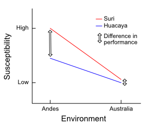
We could represent this with a graph like this:

where the huacaya geneotype performs better in the more extreme environment, but both genotypes do well in a less extreme environment.

But note how the difference between huacaya and suri performance in the Andes is greater than the difference between the same two genotypes’ performance in Australia. Thus a G × E interaction is evident, as the difference in performance between the two genotypes is also different between the two environments.

It’s important to realise that graphs of G × E interactions always have the lines converging, diverging, or even crossing. A G × E interaction does not exist if the lines are parallel. This is because there is no difference between the genotypes in different environments—each genotype has been negatively, positively, or neutrally affected equally.

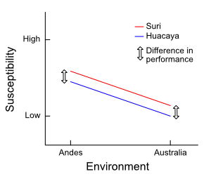
Let’s rework the graph above to make this point clearer. Again:
The following is merely to illustrate a point. It is not based on real data and in no way implies a real situation.

Here, the two lines representing susceptibility of each genotype to cold weather are parallel. In other words, the difference in performance is the same for each environment. A huacaya genotype appears equally less susceptible to cold weather than a suri genotype in both climates. There is no G × E interaction here, as both genotypes changed their performance by equal amounts when the environment changed. This graph simply describes a simple environmental effect on two genotypes, not an interaction between genotypes and environments.

You must always have at least two genotypes and at least two environments to show a genotype-environment interaction. Graphing these makes visualising the interaction so much easier. The vertical axis represents the outcome you are measuring, and the horizontal axis represents the environments you are comparing. You will have a G × E interaction only if the lines are never parallel.

The next few posts will cover more examples of graphed interactions, some real examples in the animal world, and how knowledge of G × E interactions can help develop suitable breeding objectives.

References:

1. Meat & Livestock Australia. 2016. Cattle Herd and Sheep Flock Population Changes: 2015-16 on 2012-13 percentage change. p2. Retrieved 9th February, 2018.
2. Meat & Livestock Australia. 2017. Sheep Numbers Map 2016-17. Retrieved 9th February, 2018.
3. AgriFutures Australia. 2017. Alpaca Current and Potential Growing Areas. Retrieved 9th February, 2018.
4. Vice News. 22nd July, 2016. Llamas and Alpacas are Dying because of an Unusually Cold Winter in the Andes. Retrieved 9th February, 2018.
5. Shangrilah Alpacas. 2012. Dispelling Myths About Suri. Retrieved 9th February, 2018.