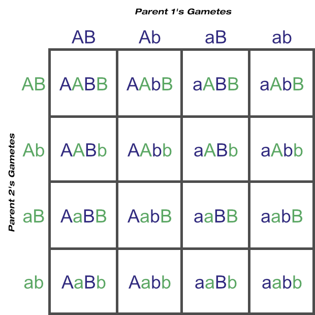
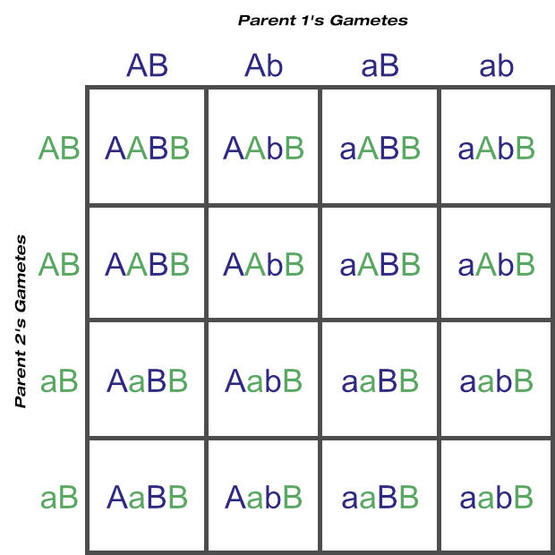
We saw earlier how chromosomes randomly assort to form sex cells during meiosis, and that the combination of chromosomes (and alleles) an organism acquires is down to which particular sperm fertilised which particular egg to make it ‘it’ and no other.
Zygote is the word for ‘fertilised egg’ in the biological/genetic worlds. A zygote is one-celled (unicellular), but through mitosis becomes a multicellular embryo, which through more mitosis and differentiation of those cells into organs and the like, develops further into a foetus until ready to be born. (It’s only natural for people to refer to foetuses so close to birth as babies or calves or puppies, but until the moment of birth they are still technically ‘foetuses’.)
So far we’ve looked at very simple models of one or two loci segregating and assorting— far too simple for the real world, but the intrinsic randomness of gene assortment could still be seen.
While this is a blog about animal breeding, let’s stick with peas a little longer as we explore this randomness further.
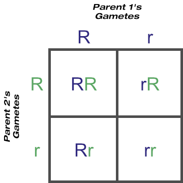
A Punnett square is a handy tool for working out the possible outcomes of a one locus mating. You’ve seen this one before, for heterozygous parents, but this time think of ‘R’ and ‘r’ as the possible gametes that can form from meiosis. Those gametes can combine in four ways:
© Optimate Group Pty Ltd
From this we can expect three-quarters of the offspring to express the dominant ’round’ trait and one-quarter to express the recessive ‘wrinkled’ trait. Statistically, the phenotype of round seed to wrinkled seed should appear in a 3:1 ratio. We’d also expect one-quarter of all offspring to be homozygous dominant, half to be heterozygous dominant, and one-quarter to be homozygous recessive. Statistically, these three unique genotypes ‘RR’, ‘Rr’ and ‘rr’ should occur in a 1:2:1 ratio.
Please note the word ’statistically’— statistics calculates the probability of an event occurring, not the certainty of it. While we may expect to see these outcomes there is no guarantee they will occur. For example, there’s a 50% chance that a baby will be a boy or a girl, which implies a family would comprise of equal numbers of boys and girls. Yet, back when larger families were the norm, it wasn’t unusual to know of ones with, say, six boys and no girls, or four girls and no boys.
Statistics work best on very large data samples, and it is usually only after many many repeated events that the observed results begin to resemble the predicted ones. Look again at Mendel’s pea data— his results that best matched the predicted 3:1 ratio were those with literally thousands of progeny. His results with ‘only’ hundreds of progeny weren’t quite as close.
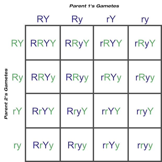
Now let’s calculate the probable outcomes of two-loci matings with a Punnett square as well, again assuming two heterozygous parents. You can see how quickly things get more complicated just by moving from four gametes to eight:
© Optimate Group Pty Ltd
Here the predicted phenotypes round and yellow:round and green:wrinkled and yellow:wrinkled and green are in a 9:3:3:1 ratio. These four phenotypes are from nine unique genotypes, in a 4:2:2:2:2:1:1:1:1 ratio.
A Punnett square could in theory be used to determine the possible gametes and genotypes from any number of loci matings, but as the above example shows, this tool doesn’t scale very well. Feel free to confirm for yourself, but just three loci would increase the number of squares to 64 (eight possible gamete combinations from each parent), and four loci would require 256 squares (sixteen possible gametes from each parent)!
There’s a much easier way to calculate the number of gametes for any number of loci — deriving a formula!
An organism heterozygous at one locus can produce two unique gametes: A and a.
An organism heterozygous at two loci can produce four unique gametes: AB, Ab, aB and ab.
An organism heterozygous at three loci can produce eight unique gametes: ABC, ABc, AbC, Abc, aBC, aBc, abC and abc.
There’s a pattern here:
1 locus, 2 unique gametes per parent if heterozygous at that locus
2 loci, 4 gametes per parent if heterozygous at each of those loci
3 loci, 8 gametes per parent if heterozygous at each of those loci
Mathematically:
21 = 2
22 = 4
23 = 8
Or, 2n = number of unique gametes, where n is the number of loci. If we plug n = 4 into this formula, we get the 24 = 2 × 2 × 2 × 2 = 16 gametes per parent mentioned above.
Now let’s work out how many unique genotypes arise from these unique gametes.
From the one-locus Punnett square above, three unique genotypes are possible if both parents are heterozygous at this locus.
From the two-locus Punnett square above, nine unique genotypes are possible if both parents are heterozygous at both loci.
And a three-locus Punnett square would reveal twenty-seven unique genotypes if both parents are heterozygous at all three loci (colour-coded here to make these slightly easier to find).

© Optimate Group Pty Ltd
Mathematically:
31 = 3
32 = 9
33 = 27
Or, 3n = number of unique genotypes, where n is the number of loci for which both parents are heterozygous.
But what if one of those parents is heterozygous at additional loci? How many unique genotypes then?
Let’s go back to locus C. If one parent is homozygous for this then it has for unique gametes: ABC, AbC, aBC and abC.
If the other parent is heterozygous then its unique gametes increase to eight: ABC, AbC, aBC, abC, ABc, Abc, aBc and abc.
Being heterozygous at one locus has enabled the number of unique gametes to double, simply because the additional ‘c’ allele increased the number of unique combinations the alleles could sort into. For every ABC there can be an ABc, and so on.
If both parents are heterozygous at two loci (A and B), there would be 32 = 9 unique genotypes from that combination alone.
But having just one parent additionally heterozygous for just one more locus © increases the unique genotypes to 18:
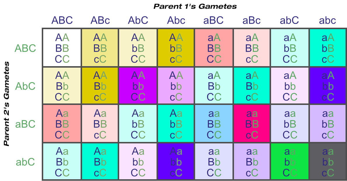
© Optimate Group Pty Ltd
I was going to delve into some more maths here but it was bogging this discussion down too much. I wrote a new post instead — for now please be satisfied that we can calculate the number of unique genotypes for any number of loci with this formula:
Number of unique genotypes = 3n × 2m where n is the number of loci both parents are heterozygous at, and m is the number of loci one parent is heterozygous at.
Another word for ‘genotype’ is zygote, our fertilised egg at the beginning of this discussion, that will ultimately grow and develop and be born as a living animal.
Thus the number of unique genotypes possible is really the number of unique zygotes possible from any union of any female and any male.
We’ve only looked at three loci so far, but animals are far more complicated that that — they are likely to have thousands or even tens of thousands of heterozygous loci.
Burt let’s assume a sire and a dam each heterozygous for 100 loci just for argument’s sake. Our formula becomes:
3n × 2m
= 3100 × 20
= 3100 × 1 (20= 1. Any number to the power of zero is one)
≅ 5 × 1047 (’≅’ means ‘approximately equal to’)
≅ 500, 000, 000, 000, 000, 000, 000, 000, 000, 000, 000, 000, 000, 000, 000, 000
≅ 500 billion billion billion billion billion unique zygotes!
That is an eye-watering number of potential offspring.
And this number is assuming there are only two alleles per locus — there are plenty of genes with three or more alleles. Of course, one parent can only ever have two of these, but it’s conceivable that four different alleles are carried between both parents. This of course just adds to the sheer randomness of it all.
Never mind that the randomness increases with additional loci! Let’s add just two more loci, that only one parent is heterozygous at:
3n × 2m
= 3100 × 22
= 3100 × 4
≅ 2 × 1048
≅ 2, 000, 000, 000, 000, 000, 000, 000, 000, 000, 000, 000, 000, 000, 000, 000, 000
≅ 2 thousand billion billion billion billion billion unique zygotes!
Mating two superior animals together does improve your chance of producing superior offspring, but because of the completely random nature of gene assortment there is no way to predict which particular combination of genes will end up in which gamete. There is no way to control which egg is fertilised by which sperm, and ultimately chance and even luck still factor in the genome you are dealt. Some gamete combinations may be so detrimental that the embryo dies very early on. Two animals who together produced a superb animal may never do so again, but at the same time a disappointing mating outcome doesn’t mean future ones will be.
So yes, there absolutely is a lot of randomness in genetic inheritance — far, far more than you may have thought. It is important to be aware of this randomness, and how, because of it, you do not have as much control over your breeding as you may think. But this is a blog about better breeding, and just knowing what you can’t control is a big step on the way to being a better breeder. We will be going deeper and deeper in our understanding, covering genes, statistics and selection strategies along the way.
But first, for completion, I do want to finish the maths touched on here — and there is now a post dedicated to just that here. After that we’ll begin a discussion on gene frequencies in populations!

